Lesson 3 - The Data Editor
In this lesson, we will explore the data editor. In particular, we’ll talk about some of the settings available for variables and viewing data in the data view.
Table of Contents
Lesson Objectives
- Learn how to use and create descriptive and data labels.
- Explore the differences between scale, ordinal, and nominal data measures.
Variable View
For the rest of this module, we’ll be working with demo.sav. If you don’t already have it open, take a moment now to do so.
Before we take a further look at our data, let’s go to the Variable View section of our Data Editor.
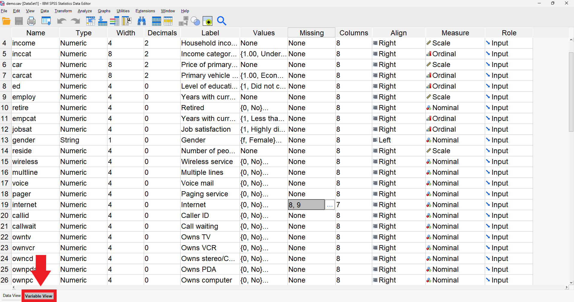
Variable Types
When creating a variable, its type is one of the most important things to define. There are several options offered, but you’ll usually be working with the Numeric and String types.
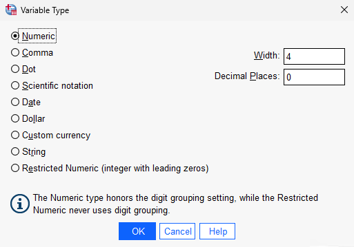
Numeric types allow for numerical input. This can be used to represent both numerical values and categorical data.
When creating numeric types, you can specify how many decimal places to use. For example, any categorical data in our datasheet has zero decimal places because we only want to be working with whole numbers.
Strings allow for character input. In this example datasheet, only gender uses the String type. However, we could use strings to store participants’ names.
When creating strings, you can specify a maximum width. The gender variable has a maximum of one character so that more characters aren’t accidentally inputted.
Descriptive Labels
As discussed in the first lesson, variables have a name and a descriptive label.
Names are short and are seen in the Data Editor, whereas labels are longer and more descriptive and are instead seen when creating plots and graphs.
Data Labels
Data labels are used to map a data value to a string label. In the example below, the numbers 1 through 5 are mapped to different levels of satisfaction.
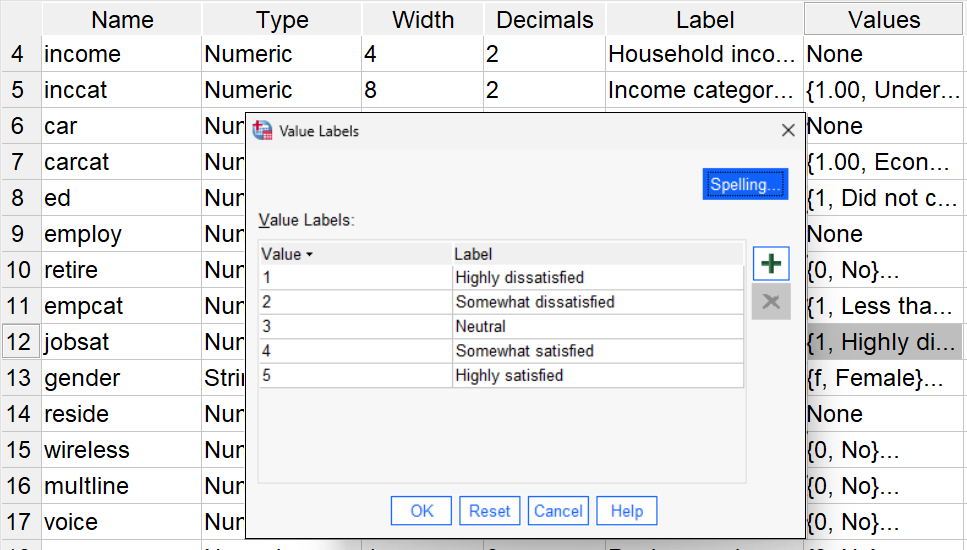
You can add more labels by clicking the + button and assigning a label to a value.
Missing Data
You can assign values to represent missing values or data that should be handled differently in analyses.
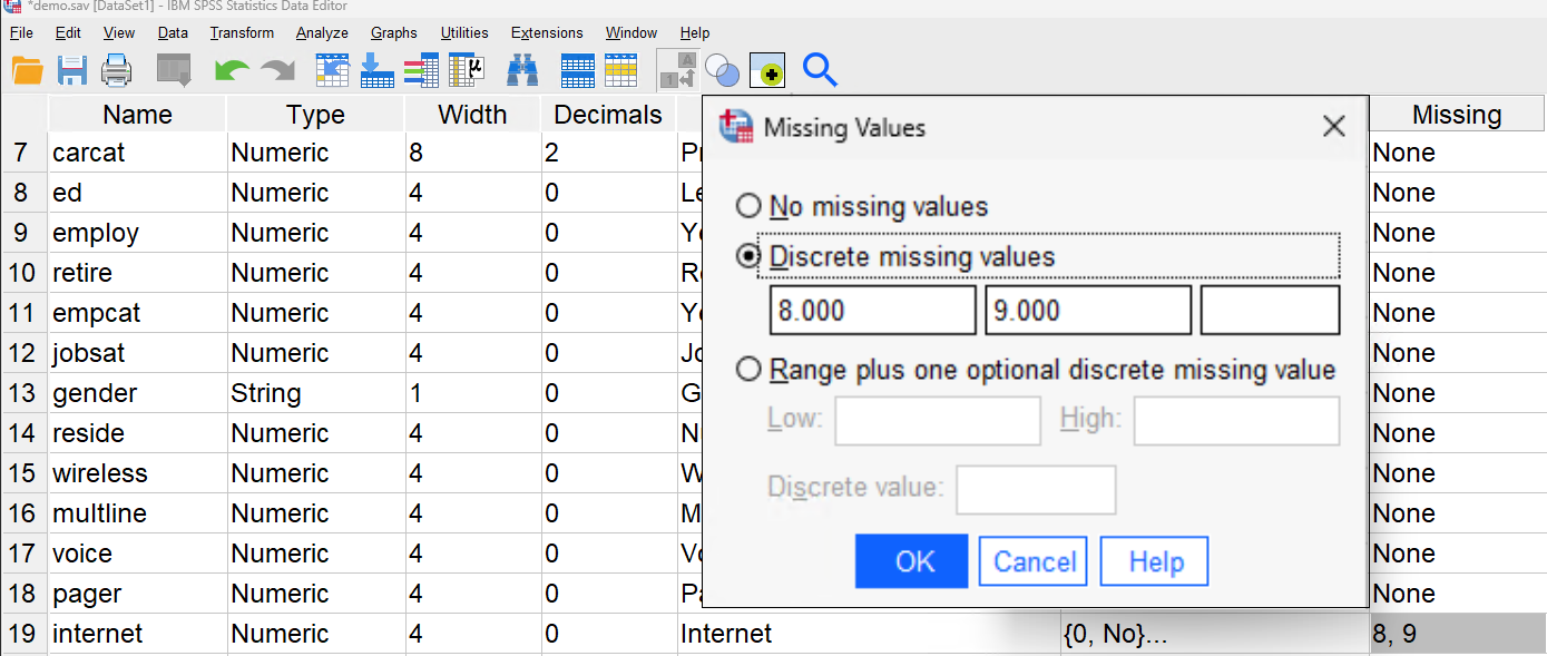
In this example, we use the discrete values 8 and 9 to represent missing data. To understand the difference between 8 and 9, we created data labels.

Here we can see that a value of 8 means that the respondent answered “I don’t know”, whereas a value of 9 represents a field that was left empty.
Variable Measure
Finally, we’ll talk about a variable’s measure type. Numeric data can have three different measure types, and it’s important to understand the differences between them.
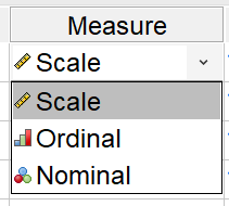
Scale: Data that can be shown on a measurement scale
Ordinal: Categorized data with an order or ranking
Nominal: Categorized data with no intrinsic order
Viewing the Data
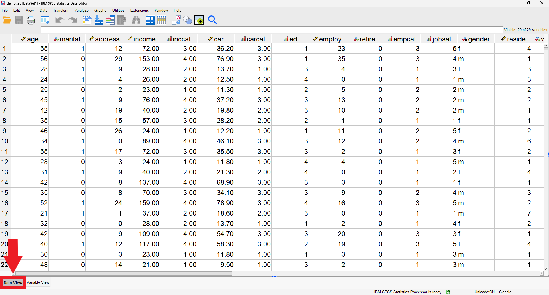
Now that we’ve talked about our variables, we can view our data. Click on the Data View button at the bottom.
The only important thing to mention here is that you’re able to toggle between displaying raw data and labelled data using the Value Labels button at the top.
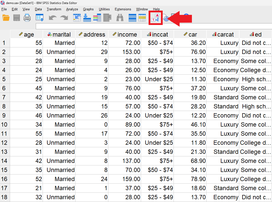
Now, instead of seeing values of 0 and 1 for marital status, we’ll get actual readable data (“Married” and “Unmarried”). You can see this with a lot of the other categorical variables too.
Key Points / Summary
- Numeric variable types are most common, but Strings are sometimes used.
- SPSS provides tools to deal with missing data.
- It’s important to understand the differences between scale, ordinal, and nominal data.
- You can use data labels in the data view to better understand your data values.